Speed of Spatial Attention
What does it mean to measure the speed of spatial attention? Within this post, we will do a small experiment using only a computer and shift the subject’s attention to parts of the screen while measuring response time. I build upon the code in Visual Search and Pop-out, and share it in appendix below.
Aim
Our task is to measure the speed of the spatial attention in the vertical vs horizontal directions, using different conditions such as delayed stimulus and smaller/larger distances.
Experimental Design
In this experiment, we will use a type of Posner cueing task, where the subject (in this case, me) is first presented with a ‘starting screen’ that introduces the key to press for input, which is chosen to be the enter key in this experiment. Upon pressing, the experiment starts with the first trial.
Trial
When the experiment starts, the subject is first presented with a ‘focus marker’ in the middle of the screen for 0.5 second. After the focus period, a cue appears in a randomised location on the screen for 0.2 second and it disappears. There is a randomly chosen delay of 100/300 ms before the appearance of the target.
The target is presented after the delay for 0.2 second and then it also disappears. Then the user is expected to press enter after seeing the target, which is recorded to be analysed.
So it is a linear process which looks like figure 1.
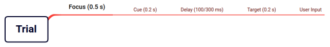 Figure 1: Trial structure
Session
In one session, a total of 1280 trials are done. These trials consist of different phases; valid/invalid trials and delays of 100/300 ms. A valid trial is a trial in which the cue and the target appear at the same location while an invalid one is where they do not (the target appears in a different location). For every location on the screen, these 2 types of trials must be equally presented. The delay between the cue and the target is also randomly changed, but the total number of both of these delays must be equal for every location, just as the trial type is.
So considering the total of 1280 trials, for a 4x4 grid size, we have 16 locations, which means 80 trials are done per location. Also considering the 4 different possible trial types (Valid-100ms, Invalid-100ms, Valid-300ms and Invalid-300ms), each of the types are presented 20 times to the subject. This is shown graphically in figure 2.
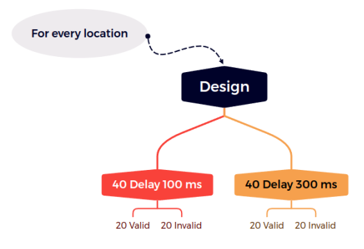 Figure 2: Location counts for different types of trials
Implementation
Scripts
The code is similar to how we organized it in Visual Search and Pop-out, and can be seen below in appendix. This time I created only 2 matlab scripts, main.m and plot_controller.m, where I implement the experimental design in main script and plot_controller just handles the plotting. You will see a straight-forward implementation; creating necessary variables, then iterating in a for-loop for the whole experiment, getting the subject input time, then saving to a matrix. Rest of the script contains helper functions for handling input events, choosing random locations for trials and the focus screen. The other script, plot_controller, handles the plotting for cue and the target plots using basic scatter plots.
Experiment
The screen is first divided into grids so that the cue can appear randomly in a given grid. Cue appearances in every grid are counted so that the cue appears with the same number on the screen locations. There is also a noise present which shifts the cue location inside the grid.
In the invalid trials, the target location is chosen randomly again with noise to move the target inside the grids (although target never moves outside its grid). The grid choice is done with weights to equally choose between different distances. What that means is euclidean distances appear with roughly the same frequencies, so the subject is presented with a ‘close’ cue and a target just as frequent as a ‘far away’ cue and a target. Of course this is present only for invalid trials since valid trials are the ones where the euclidean distance equals to zero.
In my situation, the counts of euclidean distances are shown below in figure 3, which -even if not equal - are close to each other. Note that with a larger sample size, these values would be much more close.
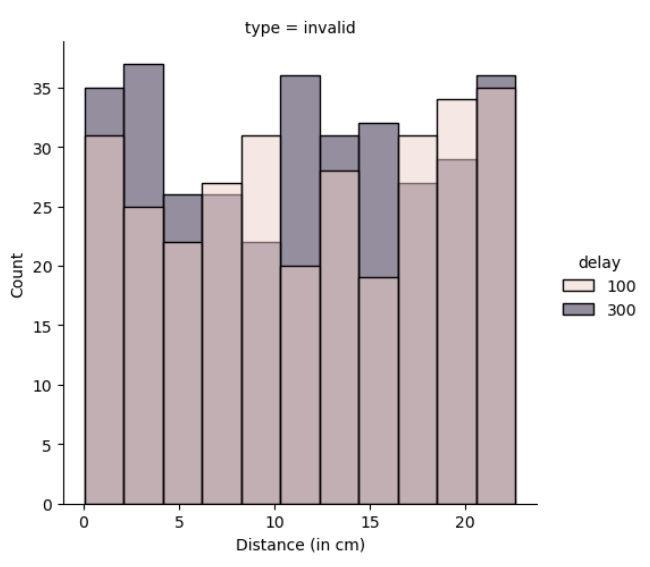 Figure 3: Counts of euclidean distances in one session
We also see in figure 3 that I have turned my units into centimetres. How I have done that is I have taken 2 points 1 unit apart in my figure, then used a ruler to measure the distance between them, and multiplied my distances in the data with that proportion, so that the analysis is done in cm rather than an arbitrary unit created in Matlab which would change with different screen size.
It is also shown in figure 3 that the delays are also presented roughly in the same counts, and their total numbers are equal. The user input time is counted with the commands tic and toc, and it is only counted after the figures are created and presented to the subject. This way, the computational time needed to prepare for the next trial is avoided to be taken into the data, and what is taken is only the subject’s reaction time.
To sum up, the subject is presented in each type of trial an equal number of times and the subject’s reaction time is measured for each type of trial, which is then analysed.
Results
The results presented here are for one subject taken in a continuous run, with the implementation described above.
Data
My data consists of 1280 rows, each row corresponding to a trial, and the columns are as follows: [‘dists’, ‘v_dists’, ‘h_dists’, ‘type’, ‘delay’, ‘times’, ‘bins’, ‘larger_bins’].
The columns that are collected during the session are ‘dists’ (euclidean distance between cue and the target), ‘v_dists’ (distance in the vertical plane), ‘h_dists’ (distance in the horizontal plane), ‘type’ (valid or invalid trial), ‘delay’ (the delay between the appearance of cue and the target) and ‘times’ (user reaction times). On the other hand, 2 more columns are added in the analysis phase, which are ‘bins’ and ‘larger_bins’, and both of them are the intervals of the distances (‘bins’ containing 23 bins and ‘larger_bins’ containing 6 bins) in order to determine the change in reaction times according to increasing distance.
The summary of the data can be shown with a violin plot, as in figure below, which at a first look, shows the different means and standard deviations for different types of trials. For example, valid trials seem to have less standard deviation compared to invalid trials. Also the highest mean seems to be in the invalid/100ms trials, which is kind of expected. Let us see statistically if these assumptions are correct, using t-tests for different groups.
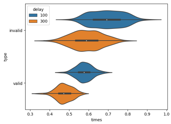 Figure 4: Violin plot of data
Difference Between Valid and Invalid Trials
Figure 5 below shows graphically the difference between valid and invalid trials, and there is a difference in terms of the mean response time. It seems that for valid trials, the reaction time is lower - which is expected since the cue and the target are presented at the same location.
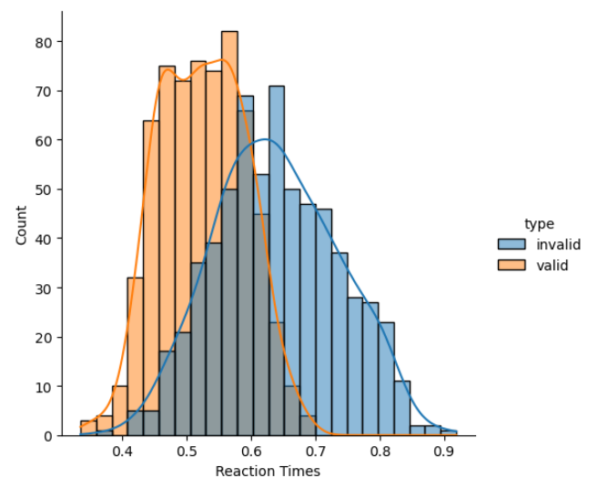 Figure 5: Difference Between Valid and Invalid Trials
We can prove the difference using a t-test (since we have 2 groups). Matlab code ‘[h,p] = ttest2(valids, invalids)’ gives ‘h=1’ for the data presented here, which means that these two groups significantly differ from each other (p<0.001).
Difference Between 100 and 300 ms Delay
What is expected beforehand for the delays, is that with a smaller delay (100 ms), the cue sometimes would not be clearly seen, so the subject reaction time might be more. Vice-a-versa, 300 ms delay is long enough to get the attention of the subject, so the subject can react to the target with a smaller reaction time.
I first plot the scatter plot for the data in hand, to see if there is a visible difference from each data. In figure 6, I believe it is clear that different delays have different reaction times, where both increase with the distance too.
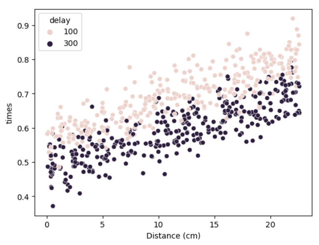 Figure 6: RT and distance compared to delays
Of course this can also be shown by a distribution plot, as in figure 7.
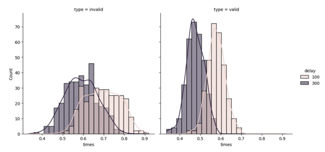 Figure 7: Distribution plot of delay times wrt different type of trials
The counts, even though seem to be different, their sums are equal for invalid and valid trials. Since the standard deviation is lower for valid trials, the counts are higher and there are lower number of bins present, hence, the steeper the curve is for the valid trials.
Note that for both of them, the curves are seemingly different; for the 100 ms delay, mean invalid trial response is around 0.6 s and mean valid response is around 0.45 s while for 300 ms delay, mean invalid response is around 0.7 s and mean valid response time is around 0.55 s. Let us again check the hypothesis that these 2 groups differ significantly, using again a t-test.
From the same matlab function, I again got ‘h = 1’ meaning that these 2 groups do differ significantly, which means that the mean response time is lower the longer the delay (p<0.001).
Difference in Response Times with respect to Euclidean Distance
Figure 5 answered the hypothesis that the reaction time of the subject would differ given a longer delay time, but it also answers the question if it would differ with increasing euclidean distance. While the data is noisy, even the scatter plot clearly shows that this hypothesis holds. Figure 8 shows this with a first degree fit line, where the slope is positive. We also see the distributions where for distances, it is approximately uniform and for reaction times, distribution approximates normal distribution.
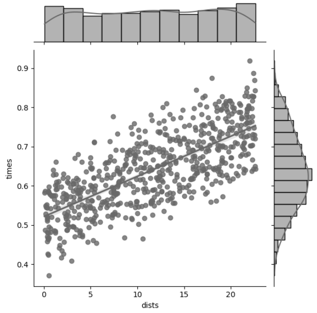 Figure 8: Conjoint plot of reaction times versus euclidean distance
In addition, we can also check vertical and horizontal distances and their respective reaction times. For that, I have created figure 9 shown below which also confirms that for an increase in any direction, the reaction time gets bigger, regardless of the delay time.
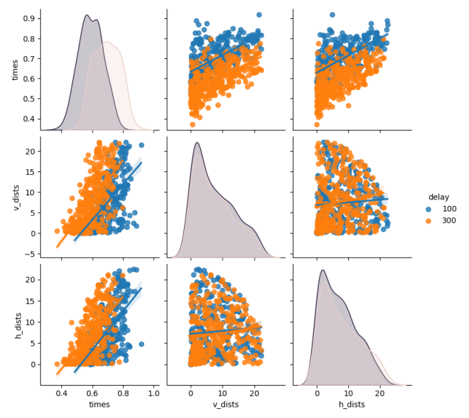 Figure 9: Reaction time vs Horizontal and Vertical Distance
The slopes are approximately equal, with values 0.93 for vertical distances and 0.97 for horizontal, meaning in this session of the experiment, vertical and horizontal searching for the target are not much different from each other.
Remember that these figures are created only for invalid trials, as for valid ones, there is no distance between cue and the target.
Speed of the Attentional Scanner
I have calculated the speed of the subject by using v = dx / dt, where I have taken only the invalid trials and so dx equals to the euclidean distance between cue and the target and dt equals to the user reaction time. For the one subject experiment explained here, I have got the result of 17.25 cm/s of attentional speed.
References
- Matlab for Neuroscientists. (2009). Elsevier. https://doi.org/10.1016/b978-0-12-374551-4.x0001-2
- Posner, M. I. (1980). “Orienting of attention”. _Quarterly Journal of Experimental Psychology doi:10.1080/00335558008248231.
Appendix
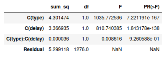
Multiple Comparisons
Multiple comparisons show us which groups differ significantly, and once again, we statistically show that trial type and delay both have significant effects on the subject reaction time (p<0.001). We also see that there is no significant interaction effect of type and delay since p is greater than 0.05.
Codes
main.m
1
2
3
4
5
6
7
8
9
10
11
12
13
14
15
16
17
18
19
20
21
22
23
24
25
26
27
28
29
30
31
32
33
34
35
36
37
38
39
40
41
42
43
44
45
46
47
48
49
50
51
52
53
54
55
56
57
58
59
60
61
62
63
64
65
66
67
68
69
70
71
72
73
74
75
76
77
78
79
80
81
82
83
84
85
86
87
88
89
90
91
92
93
94
95
96
97
98
99
100
101
102
103
104
105
106
107
108
109
110
111
112
113
114
115
116
117
118
119
120
121
122
123
124
125
126
127
128
129
130
131
132
133
134
135
136
137
138
139
140
141
142
143
144
145
146
147
148
149
150
151
152
153
154
155
156
157
158
159
160
161
162
163
164
165
166
167
168
169
170
171
172
173
174
175
176
clc;clear;clf;
% Random locs inside grids, cue disappears, limit target time
%%%%% PARAMETERS %%%%%
num_trials = 80; % For each location
grid_size = 4; % One dimension of the grid, choose even nums
points = reshape(1:grid_size^2, [grid_size grid_size]);
bounds = 0:grid_size:grid_size^2-grid_size; % Defines grids
loc_counts = repmat(num_trials/grid_size, [grid_size/2 grid_size/2 grid_size^2]);
types = ["Valid-100" "Valid-300";
        "Invalid-100" "Invalid-300"]; % This is the structure of loc_counts
total_trials = num_trials*grid_size^2;
data = ["Trial" "Subject_Time" "Subject_Answer" "Cue_Pos" "Target_Pos"];
pause_btw_events = 1; % In seconds
session_pauser = 100;

%%%%% Preadjustments %%%%%
% To make figure fullscreen, uncomment next line!
figure('units','normalized','outerposition',[0 0 1 1])
% A text before starting trial
g = text (0.3, 0.5, "Press enter to start trials");
% When enter pressed, this while will end
inp = get_input;
while inp ~= 13
    inp = get_input;
end

%%%%% Session %%%%%
for i=1:total_trials
    % Focus subject to middle
    focus_plot
    pause(0.5)
    % Choose a random location on grid
    loc = choose_loc(loc_counts, points, 0, 0);
    % Save that location's trial matrix
    curr_loc_matrix = loc_counts(:,:,loc);
    % Choose a random trial type
    trial_weights = reshape(curr_loc_matrix,1,[])/sum(sum(curr_loc_matrix));
    curr_trial = randsample(reshape(types, 1, []), 1, true, trial_weights);
    % Find plot point
    cue_point = find_plot_point(loc, points, bounds, grid_size);
    % Split trial type string for deciding target times and location
    type = split(curr_trial, "-");
    cue_point = [(2*cue_point(1)+length(bounds))/2 (2*cue_point(2)+length(bounds))/2];
    cue_point = noise(cue_point);

    % Plot
    switch type(1)
        case "Valid"
            plot_controller("Cue", bounds, cue_point)
            pause(0.2)
            empty_plot
            pause(str2double(type(2))/10^3)
            clf;
            plot_controller("Target", bounds, cue_point)
            pause(0.2)
            empty_plot
        case "Invalid"
            plot_controller("Cue", bounds, cue_point)
            pause(0.2)
            empty_plot
            pause(str2double(type(2))/10^3)
            new_loc = choose_loc(loc_counts, points, 0, loc);
            target_point = find_plot_point(new_loc, points, bounds, grid_size);
            target_point = [(2*target_point(1)+length(bounds))/2 (2*target_point(2)+length(bounds))/2];
            target_point = noise(target_point);
            clf;
            plot_controller("Target", bounds, target_point)
            pause(0.2)
            empty_plot
    end

    % Time subject
    [user_time, user_answer] = input_handler;

    % Reduce chosen trials count by 1
    trial_index = find(types==curr_trial);
    curr_loc_matrix(trial_index) = curr_loc_matrix(trial_index) - 1;
    % Overwrite 3D counts matrix with the new matrix of the trial
    loc_counts(:,:,loc) = curr_loc_matrix;

    % Store Data
    cue_entry = string(cue_point(1)) + "," + string(cue_point(2));
    if type(1) == "Valid"
        data = [data; curr_trial user_time user_answer cue_entry cue_entry];
    elseif type(1) == "Invalid"
        targ_entry = string(target_point(1)) + "," + string(target_point(2));
        data = [data; curr_trial user_time user_answer cue_entry targ_entry];
    end


    % A break every 100 trials
    if mod(i, session_pauser) == 0
        clf;
        g = text (0.3, 0.5, string(1280 - i) + " trials remaining, enter to continue");
        % When enter pressed, this while will end
        inp = get_input;
        while inp ~= 13
            inp = get_input;
        end
    end

    % Remaining trials can be shown by uncommenting next line
    %disp("Remaining trials: " + string(sum(reshape(sum(sum(loc_counts), 2), 1, []))))
end

% Save trial data
writematrix(data, string(datetime()) + "_session_data.csv")

%%%%% HELPER FUNCTIONS %%%%%
function [time, answer] = input_handler
    tic

    % space: 32, enter: 13
    k = waitforbuttonpress;
    answer = double(get(gcf,'CurrentCharacter'));

    time = toc;

    switch answer
        case 13
            answer = "Valid";
        case 32
            answer = "Invalid";
        otherwise
            answer = "Unknown_Input";
    end
end
% Input for enter skipping -> returns ASCII char of input
function inp = get_input
    k = waitforbuttonpress;
    inp = double(get(gcf,'CurrentCharacter'));
end

function loc = choose_loc(loc_counts, points, nonintersecting, old_loc)
    loc_remaining = reshape(sum(sum(loc_counts), 2), 1, []);
    loc_weights = loc_remaining/sum(loc_remaining);
    if ~(nonintersecting)
        loc = randsample(reshape(points, 1, []), 1, true, loc_weights);
    elseif nonintersecting
        while 1
            loc = randsample(reshape(points, 1, []), 1, true, loc_weights);
            if loc ~= old_loc
                break
            end
        end
    end
end

function plot_point = find_plot_point(loc, points, bounds, grid_size)
    %{
    Calculate plot location, this is needed bc 'points' array's origin is
    top left while plot grid's origin is bottom left.
    %}
    [row, column] = find(points == loc);
    plot_point = [grid_size*(column-1) bounds(end)-(grid_size*(row-1))];
end

function focus_plot
    s = scatter(8, 8, ...
            200, "+", "black");
    xlim([0 16])
    ylim([0 16])
    axis off
end

function empty_plot
    clf;
    xlim([0 16])
    ylim([0 16])
    axis off
end

% Noise to move the point inside the grid
function [noised] = noise(point)
    noised = [point(1)+rand()*4-2 point(2)+rand()*4-2];
end
plot_controller.m
1
2
3
4
5
6
7
8
9
10
11
12
13
14
15
16
17
18
19
20
21
22
23
24
25
26
27
function plot_controller(type, bounds, point)
    clf;
    % Plot the background grids
    %plot_grids(bounds)
    %hold on
    if type == "Cue"
        s = scatter(point(1), point(2), ...
            250, "x", "blue");
    elseif type == "Target"
        s = scatter(point(1), point(2), ...
            100, "red", 'filled');
    end
    xlim([0 16])
    ylim([0 16])
    axis off
    hold off
end

% Every plot will contain grids
function plot_grids(bounds)
    for j=1:length(bounds)
        for i=1:length(bounds)
            rectangle('Position', ...
                [bounds(i) bounds(j) length(bounds) length(bounds)])
        end
    end
end