Regression with Python From Scratch - Linear Regression
I try to explain a regression model with its basic math background and implement a working model from scratch using numpy only. Then, at the end, a model is created using scikit-learn framework.
Linear Regression
Linear regression is the process of writing the numeric output, called the dependent variable, as a function of the input, called the independent variable. Our assumption is, data that is to be predicted, is the sum of a deterministic function of the input and a random noise.
\[r = f(x)+\epsilon\]where r is the dependent variable, x is the independent variable and epsilon is the random noise. Using linear regression, our aim is to approximate f(x) by our estimator function.
For linear regression in one dimension, we can write our estimator as follows.
\[g(x|W_0, W_1)=W_0+W_1\cdot x\]W represent the trainable weights, which we will start randomly and change them to fit our data.
Implementation from scratch
Generating Data
Let us begin with necessary imports.
1
2
import numpy as np
import matplotlib.pyplot as plt
Now we can write any linear equation as a function and call it with our random x values.
1
2
3
4
5
def func(x):
	return 3*x + 5

X = np.random.random(1000) * 50
y = np.array([func(i) for i in X])
Adding Noise
We will add noise to y values so that it is not an exact fit, but rather closer to what we might see in any real data.
Linear regression does not assume normality on observed variables, but it assumes a 0 mean Gaussian noise on error. Even though your data might not have a normally distributed error, linear regression analysis works well with non-normal errors too. But, the problem is with p-values for hypothesis testing.
As for generating noise, it is easy using numpy. Then we add noise to our y values.
1
2
3
4
mu, sigma = 0, 10
noise = np.random.normal(mu, sigma, 1000)

y = np.add(y, noise)
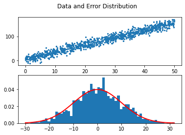
Let us show that our data is linear and the noise is Gaussian.
1
2
3
4
5
6
7
8
9
fig, axs = plt.subplots(2)
fig.suptitle('Data and Error Distribution')

axs[0].scatter(X, y, s = 5)

count, bins, ignored = plt.hist(noise, 60, density=True)
axs[1].plot(bins, 1/(sigma * np.sqrt(2 * np.pi)) *
               np.exp( - (bins - mu)**2 / (2 * sigma**2) ),
         linewidth=2, color='r')
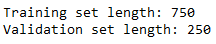
Generating Training and Validation Sets
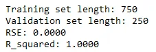
In this tutorial we go with a ratio of 2/3 to 1/3 for training and validation sets respectively. It is important to use floor division so that we do not have an indexing error.
1
2
3
4
x_tr, y_tr = np.array(X[:len(X)*3//4]), np.array(y[:len(y)*3//4])
x_val, y_val = np.array(X[len(X)*3//4:]), np.array(y[len(y)*3//4:])

print('Training set length: {}\nValidation set length: {}'.format(len(x_tr), len(x_val)))
Model Training
Random Initialization of Weights
We start by randomly generated weights. It is important to note that these weights will be trained to make our line fit our data better.
1
w0, w1 = [np.random.random() for _ in range(2)]
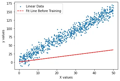
Let us see how well our randomly generated line fits our data. In order to show this fit, we need to calculate our predictions on using not yet trained weights.
1
2
3
4
5
g = w1 * x_tr + w0plt.scatter(x_tr, y_tr, s = 5, label = 'Linear Data')
plt.plot(x_tr, g, '--r', label = 'Fit Line Before Training')
plt.xlabel('X values')
plt.ylabel('y values')
plt.legend()
Updating Weights
We have our predictor as
\[g(x_i|\omega_0,\omega_1)=\omega_0+\omega_1\cdot x\]Taking the derivative of the sum of squared errors with respect to weights, we have two unknown equations.
\[\sum_i r^i = N\cdot \omega_0+\omega_1\sum_i x^i\] \[\sum_i r^i x^i=\omega_0\sum_i x^i+\omega_1\sum_i(x^i)^2\]This can be written in matrix form as
\[A\cdot W=y \rightarrow W=A^{-1}\cdot y\]where for linear regression
\[A=\begin{bmatrix} N & \sum x_i \\ \sum x_i & \sum x_i^2 \end{bmatrix}, \quad W=\begin{bmatrix} W_0 \\ W_1 \end{bmatrix}, \quad y= \begin{bmatrix} \sum y_i \\ \sum y_i\cdot x_i \end{bmatrix}\]It can now be implemented easily using numpy, and we can calculate our weights.
1
2
3
4
5
6
#Update weights
a = np.array([[len(x_tr), sum(x_tr)],
              [sum(x_tr), sum(np.square(x_tr))]])
A = np.linalg.inv(a)
w0, w1 = np.dot(A, np.array( [sum(y_tr), sum(x_tr * y_tr)] ))#Predictions
g = w1 * x_tr + w0
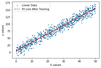
Let us plot our fitline against our data to see if our weights correctly estimate our f(x).
1
2
3
4
5
plt.scatter(x_tr, y_tr, label = 'Linear Data', s = 5)
plt.plot(x_tr, g, '--r', label = 'Fit Line After Training')
plt.xlabel('X values')
plt.ylabel('y values')
plt.legend()
Error
It seems that we are correctly representing the generated data now. But what about calculating error?
Sum of squared errors is defined as
\[E_{SSE} = \sum_{i=1}^N[r_i-g(x_i|\theta)]^2\]We want to find the $\theta$ that minimizes $E_{SSE}$. This process is called the Least Squares Estimation. By using this estimation, we can write another measure of error, which is relative square error.
\[E_{RSE} = \frac{\sum_{i=1}^N[r_i-g(x_i|\theta)]^2}{\sum_{i=1}^N[r_i-y]^2}\]We can implement this error as a function in python.
1
2
def RSE(y, g):
    sum(np.square(y - g)) / sum(np.square(y - 1 / len(y)*sum(y)))
Error now can be calculated. First we make our predictions on the validation set, then use RSE function to calculate error.
1
2
pred = lambda x, w0, w1: w1 * x + w0preds = pred(x_val, w0, w1)error = RSE(y_val, preds)
print('RSE: {}'.format(error))
which gives RSE = 0.0491.
Coefficient of Determination
A measure used to check if a regression model makes a good fit, is coefficient of determination. It can be written as
\[R^2=1-E_{RSE}\]For regression to be considered useful, we require this coefficient to be close to 1. Since we have a small error, it is clear that coefficient in our case is close to 1.
1
2
R_squared = 1 - error
print('R_squared: {:.4f}'.format(R_squared))
which gives R_squared = 0.9509.
Using Scikit-Learn for Regression
1
from sklearn.linear_model import LinearRegression as LR
Creating a regression model is rather easy using Scikit-Learn. We just call the class and fit our training data. Then we can easily see model’s scores.
1
2
3
4
5
6
7
x_tr = x_tr.reshape(-1, 1)
x_val = x_val.reshape(-1, 1)
reg = LR().fit(x_tr, y_tr)#Score model
print('Training score: ', reg.score(x_tr, y_tr))
print('Validation score: ', reg.score(x_val, y_val))#Predict specific value
predict = 30
print('Prediction for {} is: {}'.format(predict, reg.predict(np.array(predict).reshape(-1, 1))))
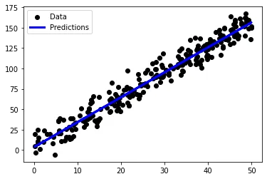
We can also visualize our predictions. First we predict values for all of validation set, then we plot it.
1
2
3
4
5
preds = reg.predict(x_val)

plt.scatter(x_val, y_val, color="black", label = "Data")
plt.plot(x_val, preds, color="blue", label = "Predictions")
plt.legend()
References
- Ethem Alpaydin. 2010. Introduction to Machine Learning (2nd. ed.). The MIT Press.
- https://data.library.virginia.edu/normality-assumption/
Appendix
Prove that if we do not add noise, our error is 0
Using the same codes written above (excluding noise)
1
2
3
4
5
6
7
8
9
10
11
12
13
14
15
16
17
18
19
20
21
22
23
24
25
26
27
28
29
def func(x):
	return 3*x + 5

X = np.random.random(1000) * 50
y = np.array([func(i) for i in X])

x_tr, y_tr = np.array(X[:len(X)*3//4]), np.array(y[:len(y)*3//4])
x_val, y_val = np.array(X[len(X)*3//4:]), np.array(y[len(y)*3//4:])

print('Training set length: {}\nValidation set length:  {}'.format(len(x_tr), len(x_val)))

w0, w1 = [np.random.random() for _ in range(2)]

#Update weights
a = np.array([[len(x_tr), sum(x_tr)],
 [sum(x_tr), sum(np.square(x_tr))]])
A = np.linalg.inv(a)
w0, w1 = np.dot(A, np.array( [sum(y_tr), sum(x_tr * y_tr)] ))

#Predictions
g = w1 * x_tr + w0
RSE = lambda y, g: sum(np.square(y - g)) / sum(np.square(y - 1 / len(y)*sum(y)))
pred = lambda x, w0, w1: w1 * x + w0
preds = pred(x_val, w0, w1)

error = RSE(y_val, preds)
print('RSE: {:.4f}'.format(error))
R_squared = 1 - error
print('R_squared: {:.4f}'.format(R_squared))
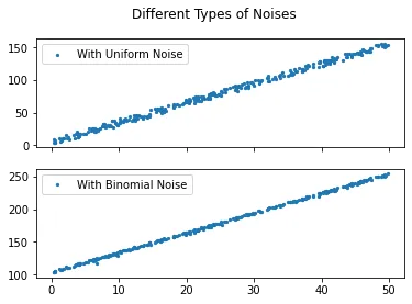
Uniform and binomial noises
1
2
3
4
5
6
7
8
9
10
11
12
13
14
15
16
17
18
19
def func(x):
	return 3*x + 5

X = np.random.random(300) * 50
y = np.array([func(i) for i in X])

noise_uni = np.random.uniform(-5, 5, 300)
n, p = 5, .3 # number of trials, probability of each trial
noise_bin = np.random.binomial(n, p, 300)

y_uni = np.add(y, noise_uni)
y_bin = np.add(y, noise_bin)

fig, axs = plt.subplots(2, sharex=True)
fig.suptitle('Different Types of Noises')
axs[0].scatter(X, y_uni, s = 5, label = 'With Uniform Noise')
axs[1].scatter(X, y_bin, s = 5, label = 'With Binomial Noise')
axs[0].legend()
axs[1].legend()