Regression with Python From Scratch - Polynomial Regression
In this story I generalize my explanations in Regression with Python From Scratch - Linear Regression post, into polynomial regression. Again starting by creating random data with noise, this time I use more of a method approach so that we can create a class for regression problems.
Polynomial Regression
Polynomial regression is a type of linear regression, known as a special case of multiple linear regression. It again makes predictions using only one independent variable, but assumes a nth degree polynomial relation between said independent variable and the dependent one.
Our assumption is also valid (just as is for linear regression) that the data that is to be predicted, is the sum of a deterministic function of the input and a random noise.
\[r = f(x)+\epsilon\]where r is the dependent variable, x is the independent variable and 𝜖 is the random noise.
Generalizing our estimator used in linear regression, we have
\[g(x|W_k,...,W_1,W_0)=W_0+W_1\cdot x+...+W_k\cdot x^k\]which can also be written as
\[g(x|W_k,...,W_1,W_0)=\sum_{i=0}^k W_i\cdot x^i\]Implementation of Polynomial Regression from Scratch
Let us start with imports.
1
2
import numpy as np
import matplotlib.pyplot as pltnp.random.seed(3)
Creating random polynomial data with noise
Generally, our function for the polynomial data can be written similarly to our estimator function.
\[f(x)=\sum_{i=0}^kc_i\cdot x^i\]where $c$ are the constants for every term in the function, and $k$ is the degree of our polynomial function.
Remember that we only write this here because we are generating the data that is going to be used in this tutorial. In a real world case, we would not know what type of function our data best fits, which is what we aim to find with our estimator function.
1
2
3
4
5
6
7
8
9
10
11
12
13
14
def func(x, c):
    return sum([c[i] * x**i for i in range(len(c))])

num_data_points = 300
degree = 3

X = np.random.uniform(-10, 10, num_data_points)
c = [np.random.uniform(-3, 3) for _ in range(degree + 1)]
y = np.array( [func(X[i], c) for i in range(num_data_points)] )

mu, sigma = 0, 50
noise = np.random.normal(mu, sigma, num_data_points)

y = np.add(y, noise)
The reason why we use degree + 1 while creating constants is that we also add a bias to our data (c_0).
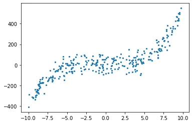
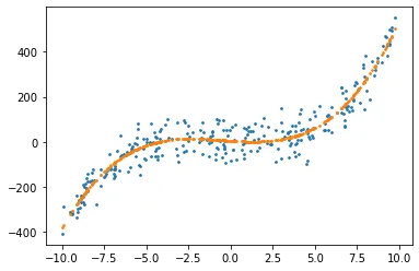
Let us plot the data.
1
plt.scatter(X, y, s = 5)
We can methodize data creation part to use easily later.
1
2
3
4
5
6
7
8
9
10
11
12
13
14
15
16
17
18
19
20
21
22
23
24
25
26
27
28
def create_poly_data(X=None, c=None, b=None,
                     degree=3, num_points=300,
                     X_lower=-10, X_higher=10,
                     c_lower=-3, c_higher=3,
                     noise=True, noise_mu=0,
                     noise_sigma=50, plot=False):

    def func(x, c):
        return sum([c[i] * x**i for i in range(len(c))])

    if X == None:
        X = np.random.uniform(X_lower, X_higher, num_points)
    if c == None:
        c = [np.random.uniform(c_lower, c_higher) for _ in range(degree + 1)]

    y = np.array( [func(X[i], c) for i in range(num_points)] )

    if noise:
        noise = np.random.normal(noise_mu, noise_sigma, num_points)
        y = [i + j for i, j in zip(y, noise)]

    if plot:
        plt.scatter(X, y, s = 5)
        plt.show()

    return X, c, y

X, c, y = create_poly_data(degree = 3, plot = True)
Generating Training and Validation Sets
1
2
3
4
x_tr, y_tr = np.array(X[:len(X)*3//4]), np.array(y[:len(y)*3//4])
x_val, y_val = np.array(X[len(X)*3//4:]), np.array(y[len(y)*3//4:])

print('Training set length: {}\nValidation set length: {}'.format(len(x_tr), len(x_val)))
Output: Training set length: 225 Validation set length: 75
Model Training
Random Initialization of Weights
We again start by initializing weights randomly.
1
W = [np.random.random() for _ in range(degree + 1)] #+1 is for W_0
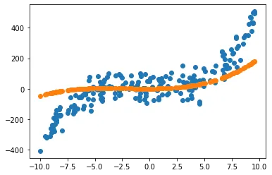
Let us plot our not yet trained estimation against our data and see how it does not make a really good fit.
Updating Weights
In order to update our weights, we are going to use the equation
\[A\cdot W=y \rightarrow W=A^{-1}\cdot y\]which is the same used for linear regression. Though now, we can generalize these matrices as follows.
\[A=\begin{bmatrix} N & \sum x_i & ... & \sum x_i^k \\ \sum x_i & \sum x_i^2 & ... & \sum x_i^{k+1} \\ .&.&.&.\\ .&.&.&.\\ \sum x_i^k & ... & ... & \sum x_i^{2k} \end{bmatrix}, \quad W=\begin{bmatrix}W_0\\W_1\\.\\.\\W_k\end{bmatrix},\quad y=\begin{bmatrix}\sum y_i\\ \sum y_i\cdot x_i\\.\\.\\ \sum y_i\cdot x_i^k\end{bmatrix}\]Notice that N is again the sum, but with 0 powers of x.
We can implement this matrix dot product as below.
1
2
3
4
5
6
7
8
9
10
11
12
def update_weights(degree, x, y):
    A = np.linalg.inv(np.array(
        [ [sum(np.power(x, i)) for i in range(j, degree + 1 + j)] for j in range(degree + 1) ]
    ))

    return np.dot(A, np.array( [ sum(y * np.power(x, i)) for i in range(degree+1) ] ))

def predict(W, x):
    return sum([W[i] * x**i for i in range(len(W))])

W = update_weights(3, x_tr, y_tr)
g = predict(W, x_tr)
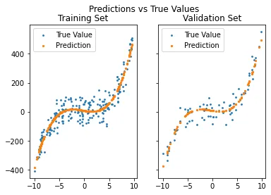
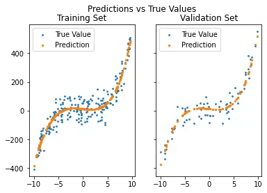
Once again we create our plot to see if this time, our predictions does fit. Let us make two plots, one to see every training data predicted, and the other for validation data.
1
2
3
4
5
6
7
8
9
10
11
12
13
14
15
16
17
18
19
def plot_predictions(x_tr, y_tr, g, x_val, y_val, g_val):
    fig, axs = plt.subplots(1, 2, sharey = True)
    fig.suptitle('Predictions vs True Values')

    axs[0].scatter(x_tr, y_tr, s = 3, label = 'True Value')
    axs[0].scatter(x_tr, g, s = 5, label = 'Prediction')
    axs[0].legend()
    axs[0].set_title('Training Set')

    axs[1].scatter(x_val, y_val, s = 3, label = 'True Value')
    axs[1].scatter(x_val, g_val, s = 5, label = 'Prediction')
    axs[1].legend()
    axs[1].set_title('Validation Set')

    plt.show()

g_val = sum([W[i] * x_val**i for i in range(len(W))])

plot_predictions(x_tr, y_tr, g, x_val, y_val, g_val)
Error and Coefficient of Determination
We are going to be using the same error that was used in linear regression, which is Relative Squared Error.
\[E_{RSE}=\frac{\sum_{i=1}^k[r_i-g(x_i|\theta)]^2}{\sum_{i=1}^k [r_i-y]^2}\]1
2
3
4
5
6
7
8
def RSE(y, g):
return sum(np.square(y - g)) / sum(np.square(y - 1 / len(y)*sum(y)))
error = RSE(y_val, g_val)
print('RSE: {}'.format(error))
R_squared = 1 - error
print('R_squared: {:.4f}'.format(R_squared))
Output: RSE: 0.0822 R_squared: 0.9178
Predicting with higher or lower degree polynomial predictors
Now let us take this a step further and see what if we assumed a 2nd degree relation between our data points and their corresponding values. We could calculate our new regressor with weights up to W squared term (remember that python range function is an open one on the upper end, meaning it does not include the upper end).
1
2
3
4
5
6
7
8
A = np.linalg.inv(np.array(
    [ [sum(np.power(x_tr, i)) for i in range(j, degree + j)] for j in range(degree) ]
))

W = np.dot(A, np.array( [ sum(y_tr * np.power(x_tr, i)) for i in range(degree) ] ))

#Predictions
g = sum([W[i] * x_tr**i for i in range(len(W))])
Which gives us the plot
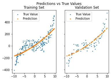
It is clear that we will have a larger error, since this fitting does a mediocre job predicting our generated values. RSE: 0.2534 R_squared: 0.7466
Or …
We could do the opposite and predict using a higher degree estimator.
1
2
3
4
5
6
7
8
9
10
degree = 6

A = np.linalg.inv(np.array(
    [ [sum(np.power(x_tr, i)) for i in range(j, degree + j)] for j in range(degree) ]
))

W = np.dot(A, np.array( [ sum(y_tr * np.power(x_tr, i)) for i in range(degree) ] ))

#Predictions
g = sum([W[i] * x_tr**i for i in range(len(W))])
This time though, we expect to have a nice fit to our data, since we expect higher degree weights to be nearly zero.
Let us see if higher degree weights are really close to zero. Printing W variable, we have

as expected.
Model Using Numpy
Numpy is too handy not to use and it has a method for calculating a fit-line. Only using one line of code (after generating our data of course), we can create a fit-line for the data.
1
2
3
4
np_model = np.poly1d(np.polyfit(X, y, 3))

plt.scatter(X, y, s = 3, label = 'Data')
plt.scatter(X, np_model(X), s = 3, label = 'Numpy Predictions')
As can be seen, we can also make predictions by passing the input data to the model.
References
- Ethem Alpaydin. 2010. Introduction to Machine Learning (2nd. ed.). The MIT Press.
Appendix
Let us put these methods into a class. I have written this class just for this purpose and not to make a library, so please note that this is of course not the best way to write this class; since there is no error handling or optimizing etc.
1
2
3
4
5
6
7
8
9
10
11
12
13
14
15
16
17
18
19
20
21
22
23
24
25
26
27
28
29
30
31
32
33
34
35
36
37
38
39
40
41
42
43
44
45
46
47
48
49
50
51
52
53
54
55
56
class regression():
    def __init__(self, degree):
        self.degree = degree

    def random_data(self, X=None, c=None, b=None,
                         degree=3, num_points=300,
                         X_lower=-10, X_higher=10,
                         c_lower=-3, c_higher=3,
                         noise=True, noise_mu=0,
                         noise_sigma=50, plot=False):

        def func(x, c):
            return sum([c[i] * x**i for i in range(len(c))])

        if X == None:
            self.X = np.random.uniform(X_lower, X_higher, num_points)
        if c == None:
            self.c = [np.random.uniform(c_lower, c_higher) for _ in range(degree + 1)]

        self.y = np.array( [func(self.X[i], self.c) for i in range(num_points)] )

        if noise:
            noise = np.random.normal(noise_mu, noise_sigma, num_points)
            self.y = [i + j for i, j in zip(self.y, noise)]

        if plot:
            plt.scatter(self.X, self.y, s = 5)
            plt.show()

        return self.X, self.y

    def split(self, X, y):
        x_tr, y_tr = np.array(X[:len(X)*3//4]), np.array(y[:len(y)*3//4])
        x_val, y_val = np.array(X[len(X)*3//4:]), np.array(y[len(y)*3//4:])

        return x_tr, y_tr, x_val, y_val

    def train(self, x, y):
        A = np.linalg.inv(np.array(
            [ [sum(np.power(x, i)) for i in range(j, self.degree + 1 + j)] for j in range(self.degree + 1) ]
        ))

        self.W = np.dot(A, np.array( [ sum(y * np.power(x, i)) for i in range(self.degree+1) ] ))

    def predict(self, x):
        self.pred = sum([self.W[i] * x**i for i in range(len(self.W))])
        return self.pred

    def plot_data_vs_estimation(self, x, y, pred):
        plt.scatter(x, y, s = 3, label = 'True Value')
        plt.scatter(x, pred, s = 5, label = 'Prediction')
        plt.legend()
        plt.show()

    def RSE(self, y, g):
        return sum(np.square(y - g)) / sum(np.square(y - 1 / len(y)*sum(y)))
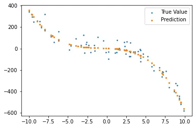
Now we can just call our methods one by one and see our regression process in action.
1
2
3
4
5
6
7
r = regression(3)
X, y = r.random_data(degree = 3, plot = True)
x_tr, y_tr, x_val, y_val = r.split(X, y)
r.train(x_tr, y_tr)
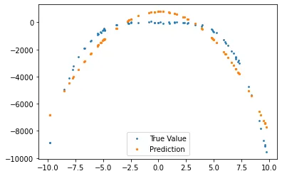
preds = r.predict(x_val)
r.plot_data_vs_estimation(x_val, y_val, preds)
print('Error: {:.2f}'.format(r.RSE(y_val, preds)))
1
Error: 0.02
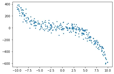
Of course we can also repeat the last part where we have used different degree predictor for the data. With our new class, it is easy to do; we only change the degree parameter while creating the random data.
1
2
3
4
5
6
7
r = regression(3)
X, y = r.random_data(degree = 4, plot = True)
x_tr, y_tr, x_val, y_val = r.split(X, y)
r.train(x_tr, y_tr)
preds = r.predict(x_val)
r.plot_data_vs_estimation(x_val, y_val, preds)
print('Error: {:.2f}'.format(r.RSE(y_val, preds)))
Error also increases: Error: 0.10