Determining Visual Thresholds - Study on Weber's Law

Ever wondered how well our eyes are able to distinguish between different luminance conditions? In this small experiment, I explore the topic of visual perception, from how we distinguish between colors to the tiny changes in brightness that catch our attention. I do the experiment myself to gather my own data, then analyze the outcome. We will discover the Weber–Fechner law and calculate the constant based on the data acquired here.

---

Aim

Here we focus on visual psychophysics and aim to measure the absolute thresholds for foveal and parafoveal vision, RGB channels and also the threshold for relative change in pixel brightness.

Experimental Design

First it is important to note that trials in this experiment should be done in a dark environment and the distance of the head to the screen should be constant. Also screen brightness should be kept the same across trials in order to avoid overall change in the brightness of the pixels.

The subject is asked to press a button if they are able to see the target, and press another button if they do not.

These being said, there are 3 experiments inside this project, where all of them have black pixels as background and there is a fixation and a target pixel on the screen with different conditions.

Foveal / Parafoveal Thresholds

We begin with comparing the thresholds for center and periphery. These trials are done with a white (or grey, since lower brightness appears to be grey) pixel. For the center, we do not put a fixation pixel and instead, right in the middle, we have the target pixel where we change the brightness.

For periphery trials, we put a fixation pixel right in the middle of the figure and then put the target pixel (which changes its brightness values) to the right of the fixation. The distance to the center is increased for every consecutive trial, so that the target is seen by different parts of the peripheral vision.

RGB Channel Thresholds

We also compare RGB channels to each other where we change the target pixel colour. Inside these trials, brightness again changes like the first trial type, but the colour is either red, green or blue. We do this trial for all three colours in separate trials to determine the thresholds for specific colours.

Note that the distance does not change between these trials and all channels are compared with the same distance.

Relative Thresholds

After determining the absolute threshold using the first task, we then put another pixel to the left of the fixation. We then ask the subject to compare the pixel on the right to the pixel on the left, and press a button if the right is brighter, or press another button if it is dimmer. By changing the distances of both of the pixels to the center pixel (or the fixation pixel), we can determine Weber’s constant, which can be calculated using the simple formula

\[W = \frac{\Delta L}{L}\]

where $\Delta L$ is the change from the standard and $L$ is the standard value of the stimulus.

Weber’s law states that the change in a stimulus that will be just noticeable is a constant ratio of the original stimulus. So the value of W should stay constant with different values of brightness of the ‘relative’ pixel.

Implementation

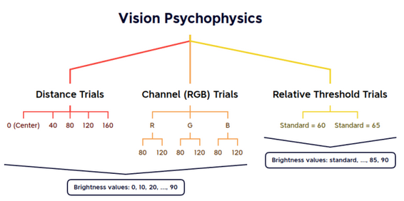Figure 1: Schema of trials of the experiment

Note that trials are done at night, without lights to create a dark environment and the subject was held at a roughly constant distance to the screen.

The codes I have written can be found below inside appendix section, where I also briefly explain them.

Foveal / Parafoveal Thresholds

To see how the threshold changes with respect to the distance to the center, for the target, I have taken distances of 0, 40, 80, 120, and 160 pixels away from the fixation pixel.

The pixel changed its brightness randomly with brightness values of 0 (no pixel shown on the figure), 10, 20, 30, 40, 50, 60, 70, 80 and 90 (10 values total) where the maximum brightness is 255. I did not need to include any value above 90 for brightness since the subject always could see the upper-range of values taken in this experiment.

I would expect for the absolute threshold to increase as the distance increases. We will see in results if that is really the case.

RGB Channel Thresholds

For the RGB channels experiment, the brightness values were just as described above, though the colour was changed to red, green and blue. So the brightness values change randomly for each colour while the fixation point is presented with a constant full brightness (of value 255 without any channels, so the colour appears white).

Trials are done in red, green and blue colour order with a constant distance of 80, then another trial for RGB channels is done with a distance of 120. It is expected for the 120 pixel distance absolute thresholds to be higher for all colour types than the 80 pixel distance.

Relative Threshold

To find the relative threshold of the subject, I presented the subject with two pixels other than the fixation one; one to the right and one to the left. Both pixels were always above the subject’s absolute threshold so that it was certain that subject always saw both pixels. Also, both of the pixels were equally distanced to the center pixel.

The brightness of the pixels changed randomly, but one of the pixels was always at the standard level of brightness. For example, if the subject is doing the trial with a standard pixel brightness of 60, then either the left or the right pixel is at brightness of 60 while the other is at a randomly chosen brightness of 60 to 90. The subject then compared these two pixels and answered whether the right is brighter or dimmer.

This trial is also repeated with distances (from the center pixel for both left and right pixels) of 80 and 120. Figure 1 shows the experiment with a schema.

Results

Foveal / Parafoveal Thresholds

First trial in this experiment answers the question ‘how does the threshold change in the periphery?’. My expectation before the trials was an increase in the absolute threshold with an increase in the distance, which is confirmed as shown below. Figure 2 shows how many times the subject reported that the target pixel is visible (as percentages) for different trials done with different distances from the fixation.

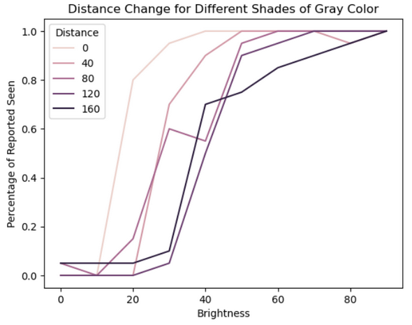Figure 2: Percentage of subject responses for different distances

Note that for 80 and 160 distance trials, 0 brightness was reported seen which is most definitely because of subject error. All of the lines do seem to have a sigmoid shape, which is expected since above a threshold must always be visible to the subject just as below a threshold value must always be invisible. Figure 3 shows sigmoid fits to the scatter plot of these data.

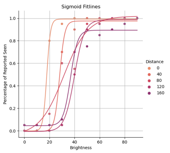Figure 3: Sigmoid fits to the distance trials data

Fitted sigmoids provide us an easy way to determine the absolute thresholds with definitive values. From these sigmoids, table 1 below is formed which shows the absolute thresholds for each distance.

Distance	0	40	80	120	160
Threshold	17.9	28.1	31.5	40.0	37.1

Table 1: Calculated absolute thresholds

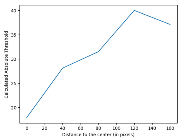Figure 3.2: Plot of calculated absolute thresholds

Table 1 and figure 3.2 shows that the presumption of increasing absolute threshold with increasing distance holds true for this experiment. It is important to note that there is a decrease in between 120 pixels distance and 160 pixels distance; which may be because of subject error, or after a distance, the absolute threshold value may also approach a limit. But to answer that question, more trials should be done with more subjects.

RGB Channel Thresholds

To determine the RGB channel thresholds, the subject - as explained above - was tested with 2 distances and all 3 channels. Figure 4 below shows the raw data plot, and from the first look, the green channel has the lower threshold while blue has the highest, for both distances.

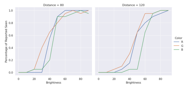Figure 4: Percentage reported seen by the subject vs brightness values for different distances of 80 and 120

Again I numerically check if that is the case by plotting a sigmoid fit to each data which can be seen below in figure 5. The sigmoid curves seem to be nicely representing the data.

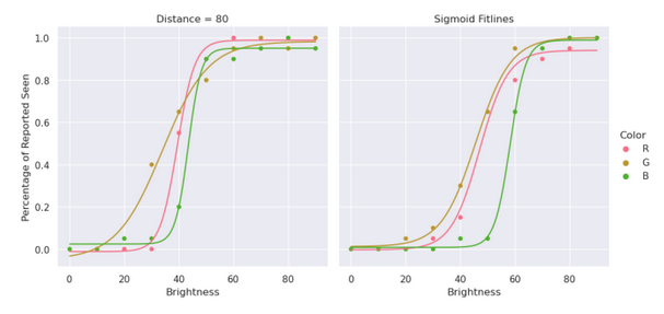Figure 5: Sigmoid fit lines for RGB channel trials data

From the sigmoid curves, 50% reported seen brightness values are gathered and put in table 2. 2 things can easily be seen in the table; threshold value increases as the distance increases -just as before- and green has the lowest threshold while blue has the highest.

Distance	Red	Green	Blue
80	39.4	34.7	43.5
120	47.4	45.3	58.1

Table 2: Calculated absolute threshold values for RGB channels

Visually, this table is shown in figure 6 as a scatter plot.

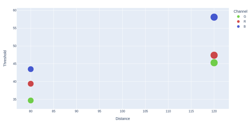Figure 6: Scatter plot of RGB channel thresholds

Relative Threshold

The procedure for finding the relative threshold is as explained above. With the same analysis steps, I have created figure 7 to show percentage detected versus difference in stimulus change (brightness change). I have also plotted the sigmoid fits.

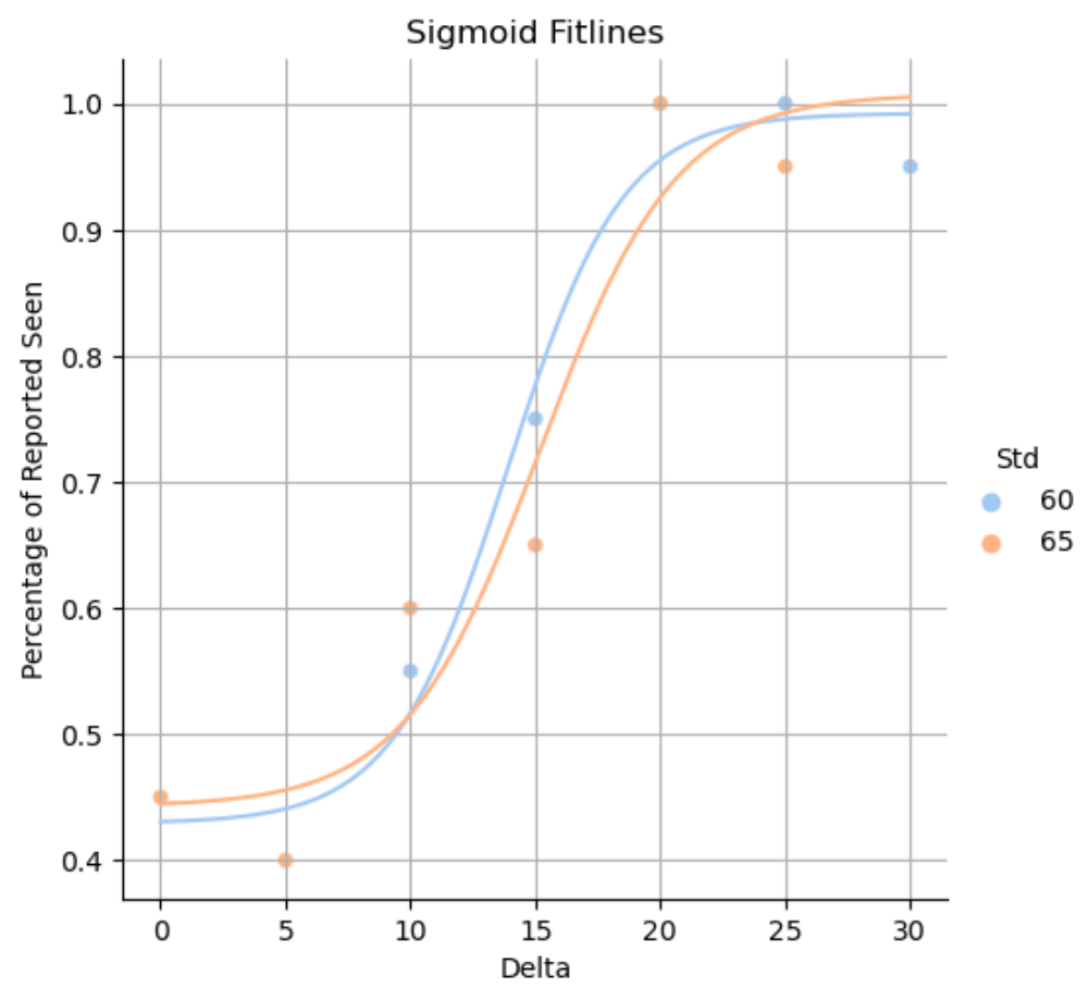Figure 7: Relative thresholds for standard values of 60 and 65 as scatter plot and their sigmoid fits as line plot

There is a clear shift to the right with a higher standard brightness. That is the expected result that on higher stimulus levels, differences should be harder to detect. Note that this dataset consists of 1 subject which is a low sample size and so it may be better to choose more separated standard values to clearly show the difference in sigmoid fit curves. The relative thresholds can be seen below in table 3.

Standard	60	65
Threshold	14.4	15.2

Table 3: Relative thresholds

We can calculate Weber’s constant from values in table 3.

\[W_1 = \frac{\Delta L}{L} = 14.4/60 = 0.240\] \[W_2 = \frac{\Delta L}{L} = 15.2/65 = 0.234\]

Even though the data is not perfect, Weber’s law seems to be close for each standard brightness value. Separation of curves in figure 7 can also be explained as being due to L getting bigger, so in order for the Weber’s constant to stay the same, ∆L should increase too. So the relative thresholds do depend on the brightness values of the dots, as can be understood symbolically from Weber’s constant too. It should increase if the standard stimulus value increases.

It does make more sense to ask the subject to identify which pixel is the brighter one because it creates a bias that one of the pixels should be brighter and the subject is pushed to tell which one. This method creates an error margin where it is reflected in the results as a sigmoid curve. It is more logical to ask to catch the difference in pixels when we are looking for the threshold for identifying the minimum stimulus to detect the difference.

References

• Matlab for Neuroscientists. (2009). Elsevier. https://doi.org/10.1016/b978-0-12-374551-4.x0001-2
• Kandel, Eric R.; Jessell, Thomas M.; Schwartz, James H.; Siegelbaum, Steven A.; Hudspeth, A. J. (2013). Principles of neural science. Kandel, Eric R. (5th ed.). ISBN 9780071390118.

Appendix

Scripts

Below are my script writtin in MATLAB for this study and the implementation is pretty straight-forward; main.m goes through the experiment stages in separate for loops for parafovial/fovial and RGB experiments, and it uses trial.m script inside the for loops. I have separated the relative thresholds experiment script, can be seen in relative.m, and it can be run separately to only do that part of the experiment.

You can run main.m for first 2 parts and relative.m for relative threshold part, to do your own experiment and then save the results, and see if you get the same outcome as we discovered here.

main.m

clc; clear; clf;

scores = ["Trial" "brightness-"+string(0:10:90)]; % List that will store all trial results

h = figure('units','normalized','outerposition',[0 0 1 1]) %Creating a figure with a handle h
set(h,'color',[0 0 0]) % Makes the figure window black

%%%%% Starting Screen %%%%%
start_text = "Press enter to continue trials";
pause_figure(start_text)

%%%%% Para/fovial experiment with shades of gray %%%%%
dists = 0:40:200; % Distances to the right from the center
for dist = dists
    pause_text = "You will be starting phase with distance " + string(dist) + ". Focus on the center.";
    pause_figure(pause_text)
    s = trial(h, dist, [1 2 3], 0); % [1 2 3] is the gray color
    scores = [scores; "Gray-"+string(dist) transpose(s)];
end

%%%%% RGB experiment %%%%%
colours = ["R" "G" "B"];
for i = 1:3 % In order, R, G and B trials are done this way
    for j = 3:4
        pause_text = "You will be starting trial with color " + colours(i) + " and with distance " + string(dists(j)) + ". Focus on the center.";
        pause_figure(pause_text)
        s = trial(h, dists(j), i, 0);
        scores = [scores; colours(i)+"-"+string(dists(j)) transpose(s)];
    end
end

% Save trial data
writematrix(scores, string(datetime()) + "_session_data.csv")

%% Helpers
function pause_figure(txt)
    clf;
    image(uint8(zeros(400,400,3)))
    text(50, 200, txt, 'Color', 'r');
    % When enter pressed, this while will end
    inp = get_input;
    while inp ~= 13
        inp = get_input;
    end
end

function inp = get_input
    k = waitforbuttonpress;
    inp = double(get(gcf,'CurrentCharacter'));
end

trial.m

function score = trial(h, dist, color, rel)
    temp = uint8(zeros(400,400,3)); %Create a dark stimulus matrix
    temp1 = cell(10,1); %Create a cell that can hold 10 matrices
    for ii = 1:10 %Filling temp1
        if dist ~= 0; temp(200,200,:) = 255; end %Inserting a fixation point
        temp(200,200+dist,color) = (ii-1)*10; %Inserting a test point dist pixels right of it. Brightness range 0 to 90.
        if rel ~= 0; temp(200,200-dist,color) = rel; end % If there is a relative distance needed, plot it
        temp1{ii} = temp; %Putting the respective modified matrix in cell
    end %Done doing that
    %h = figure('units','normalized','outerposition',[0 0 1 1]) %Creating a figure with a handle h
    %set(h,'color',[0 0 0]) % Makes the figure window black
    stimulusorder = randperm(200); %Creating a random order from 1 to 200.
    %For the 200 trials. Allows to have a precisely equal number per condition.
    stimulusorder = mod(stimulusorder,10); %Using the modulus function to create a range from 0 to 9. 20 each.
    stimulusorder = stimulusorder + 1; %Now, the range is from 1 to 10, as desired.
    score = zeros(10,1); %Keeping score. How many stimuli were reported seen
    for ii = 1:200 %200 trials, 20 per condition
        image(temp1{stimulusorder(1,ii)}) %Image the respective matrix. As designated by stimulusorder
        %ii %Give observer feedback about which trial we are in. No other feedback.
        pause; %Get the keypress
        temp2 = get(h,'CurrentCharacter'); %Get the keypress. =." for present, “,” for absent.
        temp3 = strcmp('.', temp2); %Compare strings. If . (present), temp3 = 1, otherwise 0.
        score(stimulusorder(1,ii)) = score(stimulusorder(1,ii)) + temp3 %Add up. In the respective score sheet.
    end %End the presentation of trials, after 200 have lapsed.
end

relative.m

clc; clear; clf;

scores = ["Trial" "brightness-"+string(0:10:90)]; % List that will store all trial results
rels = [40 60];
dists = [80];

h = figure('units','normalized','outerposition',[0 0 1 1]) %Creating a figure with a handle h
set(h,'color',[0 0 0]) % Makes the figure window black

%%%%% Starting Screen %%%%%
start_text = "Press enter to continue trials";
pause_figure(start_text)

for dist = dists
    for rel = rels
        s = trial_relative(h, dist, [1 2 3], rel);
        scores = [scores; 'Rel-'+string(dist)+'-'+string(rel) transpose(s)];
    end
end

function score = trial_relative(h, dist, color, rel)
    temp = uint8(zeros(400,400,3)); %Create a dark stimulus matrix
    temp1 = cell(10,1); %Create a cell that can hold 10 matrices
    for ii = 1:10 %Filling temp1
        if dist ~= 0; temp(200,200,:) = 255; end %Inserting a fixation point
        temp(200,200+dist,color) = (ii+7)*5; %Inserting a test point dist pixels right of it. Brightness range 0 to 90.
        if rel ~= 0; temp(200,200-dist,color) = rel; end % If there is a relative distance needed, plot it
        temp1{ii} = temp; %Putting the respective modified matrix in cell
    end %Done doing that
    %h = figure('units','normalized','outerposition',[0 0 1 1]) %Creating a figure with a handle h
    %set(h,'color',[0 0 0]) % Makes the figure window black
    stimulusorder = randperm(200); %Creating a random order from 1 to 200.
    %For the 200 trials. Allows to have a precisely equal number per condition.
    stimulusorder = mod(stimulusorder,10); %Using the modulus function to create a range from 0 to 9. 20 each.
    stimulusorder = stimulusorder + 1; %Now, the range is from 1 to 10, as desired.
    score = zeros(10,1); %Keeping score. How many stimuli were reported seen
    for ii = 1:200 %200 trials, 20 per condition
        image(temp1{stimulusorder(1,ii)}) %Image the respective matrix. As designated by stimulusorder
        %ii %Give observer feedback about which trial we are in. No other feedback.
        pause; %Get the keypress
        temp2 = get(h,'CurrentCharacter'); %Get the keypress. =." for present, “,” for absent.
        temp3 = strcmp('.', temp2); %Compare strings. If . (present), temp3 = 1, otherwise 0.
        score(stimulusorder(1,ii)) = score(stimulusorder(1,ii)) + temp3 %Add up. In the respective score sheet.
    end %End the presentation of trials, after 200 have lapsed.
end

%% Helpers
function pause_figure(txt)
    clf;
    image(uint8(zeros(400,400,3)))
    text(50, 200, txt, 'Color', 'r');
    % When enter pressed, this while will end
    inp = get_input;
    while inp ~= 13
        inp = get_input;
    end
end

function inp = get_input
    k = waitforbuttonpress;
    inp = double(get(gcf,'CurrentCharacter'));
end