Regression Tree From Scratch Using Python
In this story, I dive into the topic of Regression Tree and its basic mathematical background. I will try to explain it as simple as possible and create a working model using python from scratch.
I will be using recursion to create tree nodes, so if that is something you are not familiar with, I recommend looking some examples and explanations online (though I still will be explaining its logic briefly).
Imports:
1
2
3
import pandas as pd
import numpy as np
import matplotlib.pyplot as plt
Creating Data
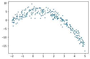
Beginning with creating a numerical data, the data will have an independent variable (x) and a dependent one (y). Using numpy, I will add a gaussian noise to dependent values, which can be expressed mathematically as
\[y=f(x)+\epsilon\]where $\epsilon$ is the noise.
Using numpy for creating a data, we can calculate dependent variable and add noise in one step as below.
1
2
3
4
5
6
7
8
9
10
11
def f(x):
    mu, sigma = 0, 1.5
    return -x**2 + x + 5 + np.random.normal(mu, sigma, 1)

num_points = 300
np.random.seed(1)

x = np.random.uniform(-2, 5, num_points)
y = np.array( [f(i) for i in x] )

plt.scatter(x, y, s = 5)
Regression Tree
Tree Structure
In a regression tree, we predict numerical data by creating a tree of multiple nodes where every training point ends up in one node. The diagram below shows an example of a tree structure for regression trees, where every node has its threshold value for dividing up the data.
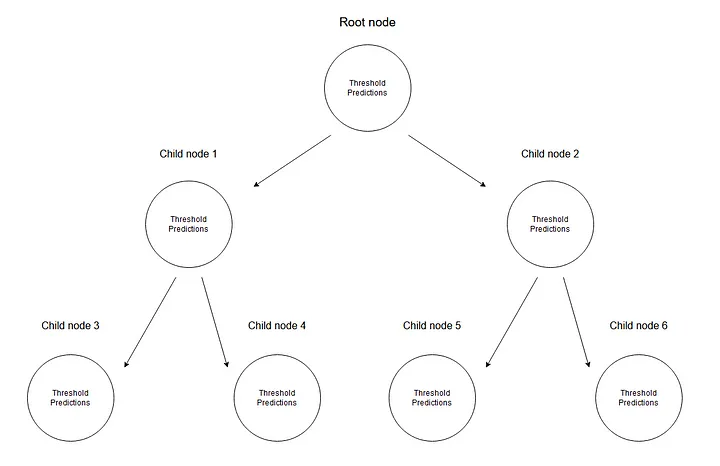
Every node stores its threshold and predictions.
Given a set of data, an input value will be reaching to a leaf. All input values of X that reaches a node m, can be represented with a subset of X. Mathematically, let us express this situation with a function which gives 1 if a given input value reaches a node m, and 0 otherwise.
\[b_m(x)=\begin{Bmatrix}1, & \mbox{if}\quad x\in X_m \\ 0, & \mbox{otherwise}\end{Bmatrix}\]Implementation from Scratch
Finding a threshold for splitting the data
We start by iterating through the sorted training data by picking 2 consecutive points at each step, and calculating their mean. The mean we calculate is the threshold value to split the data into two.
Let us take a threshold value randomly to consider any given situation.
1
2
3
4
5
6
7
8
9
10
11
threshold = 1.5

low = np.take(y, np.where(x < threshold))
high = np.take(y, np.where(x > threshold))

plt.scatter(x, y, s = 5, label = 'Data')
plt.plot([threshold]*2, [-16, 10], 'b--', label = 'Threshold line')
plt.plot([-2, threshold], [low.mean()]*2, 'r--', label = 'Left child prediction line')
plt.plot([threshold, 5], [high.mean()]*2, 'r--', label = 'Right child prediction line')
plt.plot([-2, 5], [y.mean()]*2, 'g--', label = 'Node prediction line')
plt.legend()
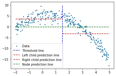
A random threshold value, with its and children node’s predictions.
Blue vertical line represent a single threshold value where we assume it is any given two point’s mean. It will be used to divide up the data later on.
Our first prediction on the problem is the mean value (of y-axis) for all training data (green horizontal line). 2 red lines are the predictions for the children node to be created.
While it is clear that none of these mean values represent our data well yet, it shows the difference; main node prediction (green line) gets the mean of all training data, but we divide it into 2 children nodes and those 2 children have their own predictions (red lines) which represents their corresponding training data a little bit better, compared to the green line. We will be constantly dividing the data into 2 — creating 2 childrens from every node until we hit a given stop value, which is the least amount of data a node can have. This is called pre-pruning the tree, where it early stops the tree construction process.
Remember: If we were to continue dividing up till we reach a single value, it would create an overfitting scenario where for each training data, its prediction would be itself.
Spoiler alert: when the model is finished, it will not predict any value using the root or any intermediate nodes; it will be predicting using the leaves of the regression tree (which will be the last nodes of the tree).
To get the threshold value which best represents the data for a given threshold, we use sum of squared residuals. It can be defined mathematically as
\[SSR=\sum_{j=1}^J \sum_i (y_i-\bar{y}_{mj})^2\cdot b_{mj}(x_i)\]Let us see in action, how this step works.
 Animation code available below in appendix.
Now that we calculated SSR values for thresholds, we can take the threshold that has the minimum SSR value. This threshold will be used to divide the training data into two — a low and a high part — where the low one will be used to create the left children node, and the high will contribute in creating the right one.
1
2
3
4
5
6
7
8
9
10
11
12
13
14
15
16
17
18
def SSR(r, y):
    return np.sum( (r - y)**2 )

SSRs, thresholds = [], []
for i in range(len(x) - 1):
    threshold = x[i:i+2].mean()

    low = np.take(y, np.where(x < threshold))
    high = np.take(y, np.where(x > threshold))

    guess_low = low.mean()
    guess_high = high.mean()

    SSRs.append(SSR(low, guess_low) + SSR(high, guess_high))
    thresholds.append(threshold)

print('Minimum residual is: {:.2f}'.format(min(SSRs)))
print('Corresponding threshold value is: {:.4f}'.format(thresholds[SSRs.index(min(SSRs))]))
Output:
1
2
	Minimum residual is: 2527.33
	Corresponding threshold value is: 3.3239
Before going into the next step, I will use pandas to create a dataframe and will create a method for finding the best threshold. All these steps could be done without pandas, it is just a personal choice to use it.
1
2
3
4
5
6
7
8
9
10
11
12
13
14
15
16
17
18
19
20
21
df = pd.DataFrame(zip(x, y.squeeze()), columns = ['x', 'y'])

def find_threshold(df, plot = False):
    SSRs, thresholds = [], []
    for i in range(len(df) - 1):
        threshold = df.x[i:i+2].mean()

        low = df[(df.x <= threshold)]
        high = df[(df.x > threshold)]

        guess_low = low.y.mean()
        guess_high = high.y.mean()

        SSRs.append(SSR(low.y.to_numpy(), guess_low) + SSR(high.y.to_numpy(), guess_high))
        thresholds.append(threshold)

    if plot:
        plt.scatter(thresholds, SSRs, s = 3)
        plt.show()

    return thresholds[SSRs.index(min(SSRs))]
Creating children nodes
Now that we have split our data into two, we can find seperate thresholds for both the low values and high values. Though note that we need a stopping condition; since with every node, the points in the dataset which belongs to a node gets smaller, we define a minimum number of data points for every node. If we were not to do this, every node would predict using only 1 training value, resulting in an overfitting.
We can create our nodes recursively. For that, we define a class named TreeNode which will store every value a node should. After that, we create the root first, while calculating its threshold and prediction values. Then we recursively create its children nodes, where every children node class is stored as an attribute of its parent class, either named left or right.
In create_nodes method, we start by splitting the given dataframe into two parts; low and high, using that node’s threshold. Then we check if there is enough data points to create left and right nodes in seperate if conditions, by using their corresponding dataframes. If there are (for either one) enough data points, we calculate threshold value for its dataframe, create a child node with it and call create_nodes method again with this new node as our tree.
1
2
3
4
5
6
7
8
9
10
11
12
13
14
15
16
17
18
19
20
21
22
23
24
25
class TreeNode():
    def __init__(self, threshold, pred):
        self.threshold = threshold
        self.pred = pred
        self.left = None
        self.right = None

def create_nodes(tree, df, stop):
    low = df[df.x <= tree.threshold]
    high = df[df.x > tree.threshold]

    if len(low) > stop:
        threshold = find_threshold(low)
        tree.left = TreeNode(threshold, low.y.mean())
        create_nodes(tree.left, low, stop)

    if len(high) > stop:
        threshold = find_threshold(high)
        tree.right = TreeNode(threshold, high.y.mean())
        create_nodes(tree.right, high, stop)

threshold = find_threshold(df)
tree = TreeNode(threshold, df.y.mean())

create_nodes(tree, df, 5)
Note that this method makes its changes on the first tree provided to it, so it does not require to return anything.
Also note that while this is not usually how a recursive function is written (no return), we do not require a return since when no if statement is activated, method will return itself.
We can now check this tree structure to see if it created some nodes to fit the data better. I will manually select first 2 nodes and its predictions towards the root’s threshold.
1
2
3
4
5
6
7
8
9
10
11
12
13
14
15
16
plt.scatter(x, y, s = 0.5, label = 'Data')
plt.plot([tree.threshold]*2, [-16, 10], 'r--',
         label = 'Root threshold')
plt.plot([tree.right.threshold]*2, [-16, 10], 'g--',
         label = 'Right node threshold')
plt.plot([tree.threshold, tree.right.threshold],
         [tree.right.left.pred]*2,
         'g', label = 'Right node prediction')
plt.plot([tree.left.threshold]*2, [-16, 10], 'm--',
         label = 'Left node threshold')
plt.plot([tree.left.threshold, tree.threshold],
         [tree.left.right.pred]*2,
         'm', label = 'Left node prediction')
plt.plot([tree.left.left.threshold]*2, [-16, 10], 'k--',
         label = 'Second Left node threshold')
plt.legend()
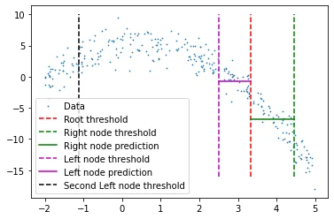
We see 2 predictions here:
- First left node’s predictions for high values (higher than its threshold)
- First right node’s predications for low values (lower than its threshold)
I have cut the prediction lines’ widths manually, which is because if a given x value reaches either of those nodes, it will be represented by the mean of all x values that belong to that node, which also means that no other x value participates in the prediction of that node (hope that makes sense).
Of course this tree structure goes much deeper than just 2 nodes. In fact, we can check a specific leaf by calling its children as follows.
1
tree.left.right.left.left

This of course means that there is a branch going down 4 children long here, but it can go much deeper on a different branch of the tree.
Predicting
We can create a prediction method to predict any given value.
1
2
3
4
5
6
7
8
9
10
11
12
13
14
def predict(x):
    curr_node = tree
    result = None
    while True:
        if x <= curr_node.threshold:
            if curr_node.left: curr_node = curr_node.left
            else:
                break
        elif x > curr_node.threshold:
            if curr_node.right: curr_node = curr_node.right
            else:
                break

    return curr_node.pred
What we do here is go down the tree by comparing every leaf’s threshold value with our input. If input is bigger than the threshold value, we go to the right leaf, and if it is smaller, then we go left, and so on until we reach to any bottom leaf. Finally we predict using that node’s own prediction value, with a final comparison with its threshold.
Testing with x = 3 (real value can be calculated using the function we have written above, while creating our data. -3**2+3+5 = -1, which is the expected value) , we get:
1
predict(3)
Output:
1
-1.2374
Calculating Error
We can use relative squared error
\[E_{RSE}=\frac{\sum_{i=1}^k[r_i-g(x_i|\theta)]^2}{\sum_{i=1}^k [r_i-y]^2}\]and create validation data as above using the same function.
1
2
3
4
5
6
7
8
9
10
def RSE(y, g):
    return sum(np.square(y - g)) / sum(np.square(y - 1 / len(y)*sum(y)))

x_val = np.random.uniform(-2, 5, 50)
y_val = np.array( [f(i) for i in x_val] ).squeeze()

tr_preds = np.array( [predict(i) for i in df.x] )
val_preds = np.array( [predict(i) for i in x_val] )
print('Training error: {:.4f}'.format(RSE(df.y, tr_preds)))
print('Validation error: {:.4f}'.format(RSE(y_val, val_preds)))
Output:
1
2
	Training error: 0.0358
	Validation error: 0.0595
which is arguably a low error.
Generalizing the steps

Appendix
A better suited data for a regression tree model
The data that I have chosen was a polynomial one and it could better be fit using a polynomial regression model. Though we could easily see a dataset where a regression tree model would work much better than a standard regression. Let me take our new function as \(y=\begin{Bmatrix}1+\epsilon, & \mbox{if} & x<3 \\ 9+\epsilon, & \mbox{if} & 3<x<6 \\ 5+\epsilon, & \mbox{if} & 6<x\end{Bmatrix}\) Implementation and visualization:
1
2
3
4
5
6
7
8
9
10
11
12
def f(x):
    mu, sigma = 0, 0.5
    if x < 3: return 1 + np.random.normal(mu, sigma, 1)
    elif x >= 3 and x < 6: return 9 + np.random.normal(mu, sigma, 1)
    elif x >= 6: return 5 + np.random.normal(mu, sigma, 1)

np.random.seed(1)

x = np.random.uniform(0, 10, num_points)
y = np.array( [f(i) for i in x] )

plt.scatter(x, y, s = 5)
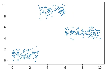
I have ran all the same process above for this dataset, which gave the error values of
1
2
	Training error: 0.0265
	Validation error: 0.0286
which are lower than the error we got from the polynomial data.
Code for the animated plot
1
2
3
4
5
6
7
8
9
10
11
12
13
14
15
16
17
18
19
20
21
22
23
24
25
26
27
28
29
30
31
32
33
34
35
36
37
38
39
40
41
42
43
44
45
46
47
48
49
50
51
52
53
54
55
56
57
58
59
60
61
62
63
64
65
66
67
68
import pandas as pd
import numpy as np
import matplotlib.pyplot as plt
from matplotlib.animation import FuncAnimation

#===================================================Create Data
def f(x):
    mu, sigma = 0, 1.5
    return -x**2 + x + 5 + np.random.normal(mu, sigma, 1)

np.random.seed(1)

x = np.random.uniform(-2, 5, 300)
y = np.array( [f(i) for i in x] )

p = x.argsort()
x = x[p]
y = y[p]


#===================================================Calculate Thresholds
def SSR(r, y): #send numpy array
    return np.sum( (r - y)**2 )

SSRs, thresholds = [], []
for i in range(len(x) - 1):
    threshold = x[i:i+2].mean()

    low = np.take(y, np.where(x < threshold))
    high = np.take(y, np.where(x > threshold))

    guess_low = low.mean()
    guess_high = high.mean()

    SSRs.append(SSR(low, guess_low) + SSR(high, guess_high))
    thresholds.append(threshold)

#===================================================Animated Plot
fig, (ax1, ax2) = plt.subplots(2,1, sharex = True)
x_data, y_data = [], []
x_data2, y_data2 = [], []
ln, = ax1.plot([], [], 'r--')
ln2, = ax2.plot(thresholds, SSRs, 'ro', markersize = 2)
line = [ln, ln2]

def init():
    ax1.scatter(x, y, s = 3)
    ax1.title.set_text('Trying Different Thresholds')
    ax2.title.set_text('Threshold vs SSR')
    ax1.set_ylabel('y values')
    ax2.set_xlabel('Threshold')
    ax2.set_ylabel('SSR')
    return line

def update(frame):
    x_data = [x[frame:frame+2].mean()] * 2
    y_data = [min(y), max(y)]
    line[0].set_data(x_data, y_data)

    x_data2.append(thresholds[frame])
    y_data2.append(SSRs[frame])
    line[1].set_data(x_data2, y_data2)
    return line

ani = FuncAnimation(fig, update, frames = 298,
                    init_func = init, blit = True)
plt.show()
#ani.save('regression_tree_thresholds_120.gif', writer='imagemagick', fps=120)